
New Hampton School, 70 Main Street, New Hampton, New Hampshire, USA
Mentor, Dr. William H. Waller, IAU/OAE/US-NAEC, 243 Granite Street, Rockport, MA, USA
Abstract
Auroras are caused by disturbances in the Earth’s magnetosphere that are produced by the variable solar wind. The connection between the magnetospheric disturbances at high altitude and the aurora phenomena at lower altitudes remains incomplete. The formula for collisional excitation of the atoms responsible for auroral emission can explain why green auroras from excited oxygen atoms can occur at relatively low altitudes, but red auroras from these same atoms are constrained to higher altitudes of lower density. The same formula also suggests much lower electron velocities (~100 km/s) than are required to excite the oxygen atoms to the required metastable levels for subsequent emission (~1000 km/s). Observations of the [OI] 630 nm spectral line profile support these low electron velocities. Other observations at higher altitude plus laboratory simulations point to much higher electron velocities of 20,000 km/s that would require significant acceleration by Alfvén waves.
Keywords
Aurora, Auroral Acceleration, Plasma, Alfvén Waves, Collisional Excitation, Ionosphere
1. Introduction:
1.1 Aurora basics
Auroras, also called polar lights, northern lights or southern lights, are natural luminous spectacles. Most auroras appear in higher-latitude regions, within an interval called “the aurora zone”, which is 3° to 6° wide in latitude and between 10° and 20° from the geomagnetic poles, and is most clearly seen at night (see Figure 1). Early evidence for a geomagnetic connection was noticed due to the statistical correlations between geomagnetic events and auroral observations. Auroras are caused by disturbances in the Earth’s magnetosphere that are produced by the variable solar wind. Trajectories of the charged particles, mainly electrons and protons, in the magnetospheric plasma, are altered by these magnetohydrodynamic (MHD) disturbances. The resulting collisional ionization and excitation of the atmospheric gases at altitudes of 100-300 km leads to the emission of light of various colors and complexity. The form of auroras is dependent on the amount of acceleration imparted to the exciting particles. Auroras were also discovered in many planets, natural satellites, brown dwarfs, and even comets in the solar system. [1]

1.2 Basic observations and proposed causes
Aurora was named after the Roman goddess of morning, Aurora, when Galileo Galilei coined the term “aurora borealis” as early as 1619 A.D.. He had the misconception that the auroras were a result of sunlight reflecting from the atmosphere. In 1790, Henry Cavendish made quantifiable observations of the aurora by using triangulation to estimate that the auroral light is produced around 100-130 km in altitude (about 60 miles above Earth’s surface). In 1902-1903 Kristian Birkeland, a Norwegian physicist, made his conclusion from his “terrella experiment” that auroral light was the result of currents flowing through the gas of upper atmosphere.[2]
While the color of auroras varies, the cause also shifts. Red auroras are usually seen at the highest altitudes (200-500 km), where excited atomic oxygen emits at 630 nm (red). The lower concentration of atoms lead to less emissions, and the lower sensitivity of our eyes towards red make this color visible only under intense solar activity. When it comes to lower altitudes (100 km or less), more frequent collisions suppress the 630 nm (red) mode, and so the auroral display is dominated by the 557.7 nm emission (green). These changes are consistent with the “forbidden” nature of the atomic emissions, where electronic transitions from their excited metastable states can be quenched by collisional de-excitations (see Figure 2).

For example, the red [OI] emission at 630 nm wavelength involves an electronic transition from the atom’s longest-lived metastable state (with a 107s spontaneous transition time) and so is most subject to quenching via collisional de-excitations. Only at the higher, less-dense altitudes can it effectively radiate. By contrast, the green [OI] emission at 557.7 nm wavelength has a much shorter spontaneous transition time of 0.7 s and so can make the jump and radiate despite the higher-density and higher collisional-rate environments that prevail at lower altitudes. The higher concentration of atomic oxygen at these altitudes and greater eye sensitivity in green lead to the common appearance of green auroras (see Figure 3).

Excited molecular nitrogen also contributes to the observed green color. It can transfer the energy by collision to an oxygen atom, which then radiates the energy away emitting the color of green. Sometimes red and green also mix together to produce auroras with rarely seen colors such as pink or yellow. As altitude increases and density decreases, atomic oxygen becomes uncommon, and molecular nitrogen and ionized molecular nitrogen dominate in producing visible light emission, radiating at a large number of wavelengths in both the red and blue parts of the spectrum, with 428 nm (blue) taken over. Blue and purple emissions appear at the highest levels of solar activity. Compared with the atomic oxygen transitions, molecular nitrogen transitions are much faster.[4]
1.3 Modeling auroras
Auroras are caused by multiple factors, including direct collisional excitation of atmospheric gases by electrons which are thought to have “precipitated” downward from the magnetosphere, where they had been accelerated to 20,000 km/s speeds via MHD waves such as Alfvén waves. A thorough understanding of the electronic cascade leading to different types of auroras is still incomplete, yet most models invoke the interaction of the solar wind with the magnetosphere. The Alfvén wave model, a theory first introduced in 1946 by Russian physicist, Lev Landau, could provide a major key to the excitation of auroral gases.[6] These waves could accelerate charged particles toward Earth’s lower atmospheric altitudes, thereby exciting the ambient oxygen and nitrogen atoms at these altitudes to sufficient energies for subsequent emission. The Alfvén wave refers to the type of magnetohydrodynamic (MHD) wave in which charged particles oscillate due to a restoring force provided by an effective tension on the magnetic field lines. The formula used to calculate the speed of Alfvén waves is stated below:

where

Here V is the phase velocity of the wave, VA is the Alfvén wave group velocity, c is the speed of light, B is the magnetic field strength, μ0 is the permeability of the vacuum, and ρ is the mass density. [5]
For example, typical magnetospheric values of B ~ (50-100) x 10-9 Teslas, n(ion) ~ 1/cm3 ⇒ ρ(ion) ~2.7 x 10⁻²⁰ kg/m3, and μo = 1.257 x 10⁻⁶ m kg s-2 A-2 will yield an Alfven speed of VA = 270 – 540 km/s. Kim, Kim, and Kwon (2018), using data from the Themis satellite, got slightly higher values of VA = 400 – 800 km/s, where their density referred to an average amu that was smaller (3) than what I used assuming all oxygen (amu = 16). [6]
A simulation of electron acceleration via Alfvén waves was completed in a lab at the Large Plasma Device (LPD) in UCLA’s Basic Plasma Science Facility recently, and the measurement matched the predictions from a computer simulation and associated mathematical calculations. According to the description by Greg Howes, co-author of the study, “Measurements revealed this small population of electrons undergoes ‘resonant acceleration’ by the Alfvén wave’s electric field, similar to a surfer catching a wave and being continually accelerated as the surfer moves along with the wave,” and that “Alfvén waves can accelerate the electrons (up to speeds of 45 million miles per hour, which is about 72 million kilometers per hour) that cause the aurora.” [7]
1.4 Research goals and strategies
The first question I will address is whether or not the forbidden [OI] emission properties can be understood in terms of modeled collision probabilities vs. transition probabilities within the changing auroral environment. Here, I intend to quantitatively explain the altitude dependence of the green vs. red [OI] emissions with reference to the quantum states of these transitions.
The second question I will address is what sorts of electronic speeds are evident from the auroral phenomena themselves? I will focus on the Doppler-broadened 630 nm spectral line of [OI] observed at high-resolution. From this measurement, I derive the velocity dispersion of the oxygen atom and then infer the velocity dispersion of the colliding electrons. That quantification will determine whether or not additional acceleration of the electrons (beyond what the solar wind provides) is necessary. This determination is key to assessing the relevance of the Alfvén wave model — and to further assess the emission properties that were quantified in addressing the first question. This latter assessment leads to a discrepancy that is discussed further in the Conclusions.
2. Modeling
2.1 Plausible modeling of Alfvén wave electron acceleration
As mentioned earlier in the Introduction, the aurora phenomenon has a high dependence on spectral-line emissions from atomic oxygen. Below is the energy level diagram of atomic oxygen showing different spectroscopic transitions, from where I acquired my data.

Red auroras are usually observed at the higher altitudes of about 200 km, where excited atomic oxygen emits at 630 nm (red). For such emissions, the excitation energy Ee equals 1.96 eV. This should equal the kinetic energy that is transferred to the oxygen atom by charged particles, mainly electrons. The velocity of the electrons, therefore, would be Ve = √(2 x K.E./me) = √(2(1.602 x 10⁻¹⁹)(1.96)/me)= 830 km/s. Based on a similar calculation, the excitation energy from the ground state to the metastable level for green 557.7 nm emission, which usually occurs at lower altitudes, is Ee = 4.19 eV, and the velocity of the exciting electrons leading to the emission is Ve = 1214 km/s.
Compared with the speed of the solar wind, usually between 300 and 700 km/s, there must be other acceleration mechanisms responsible for the inferred exciting electron velocities, such as Alfvén waves. Scientists have demonstrated in the laboratory that Alfvén waves can accelerate the electrons to as much as 45 million miles per hour, which is about 72 million kilometers per hour or 20,000 km/s, far above the threshold of 200-700 km/s provided by the solar wind, meaning that such Alfvén waves could be possible for the necessary acceleration. Recent direct detections of such high-energy electrons in Earth’s magnetosphere have been made by the Japanese Exploration of Energization and Radiation in Geospace (ERG) satellite.[9][10] In this paper we present evidence for “secondary low energy electrons” with energies much less than 1 keV at the lower auroral altitudes.
2.2 Modeled collision probabilities vs. transition probabilities
Collisional excitation and transitional de-excitation (with the emission of a photon) are two mechanisms for changing the energy of an electron that is bound in an atom. In the case of auroras, collisional excitation is the major cause of the excitation of atomic oxygen’s electrons to higher energy levels. The rate of collisional excitation should not greatly exceed the transition probability. Otherwise the collisions will de-excite the electron before it has a chance to make its photonic transition. The formula to calculate the probability for collisional excitation is Pc = n σ v, where Pc is the probability of collisions (in units of collisions/s), n is the density of particles (in units of particles/cm3) in this case atomic oxygen, σ is the cross-sectional area of interaction (in units of cm2), and v is the velocity of the colliding particles (in units of cm/s). In the next step, I’ll calculate the probability for the collisional excitation of [OI] at altitudes of 100 km (favoring the green emission) and 200 km (favoring the red emission).
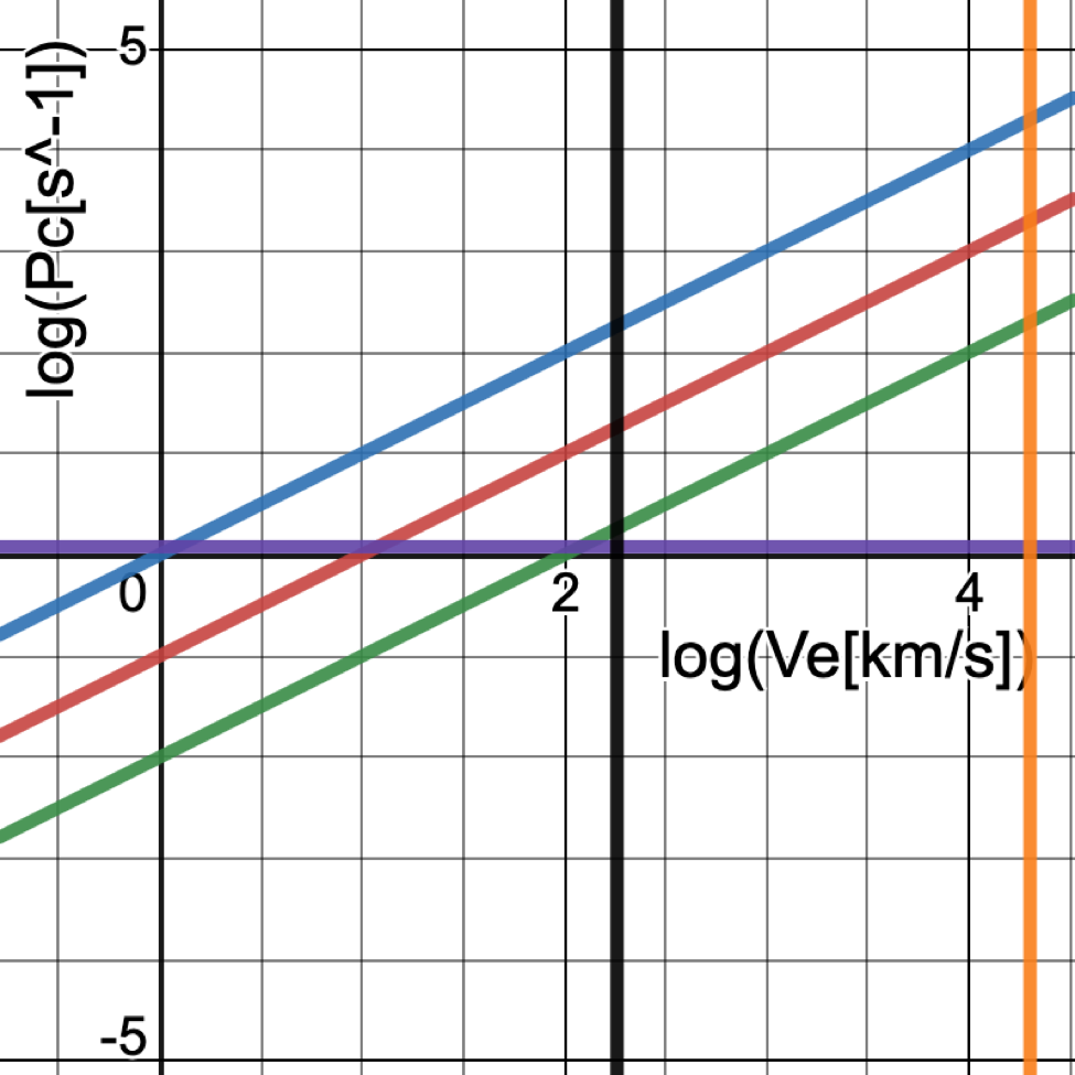
FIGURE 5(a): Relation between collision probability (Pc) and electron velocity (Ve) for different interaction cross sections (σ) of 10-19(green), 10-18(red), and 10-17(blue) cm2 in log-log format for the atmospheric situation at 100 km altitude. The horizontal line (purple) corresponds to Pc = Pt = 1.2 s-1 for an altitude of 100 km and corresponding density of 1012. Two vertical lines (black and orange) respectively correspond to Ve = 182 km/s as found from the [OI] spectral line and Ve = 20,000 km/s as indicated by magnetospheric observations cited by the Alfven-wave modelers. The lower-velocity line intersects the choices for sigma at values of Pc that are 1-100 times Pt, with the likely value of log(σ) = -18 (red) having Pc about 10 times greater than Pt, falling within the acceptable range. The higher-velocity line intersects the choices at values of Pc that are 100-10,000 times greater than Pt which should be unfeasible.

The horizontal line (purple) corresponds to Pc = Pt = 6.3 x 10⁻³ for the red emission line of [OI]. The vertical lines (black and orange) are respectively from the [OI] spectral line measurement and magnetospheric observations cited by the Alfven-wave modelers. The intersection of the lower-velocity line with the choices for σ yields Pc values that are 1-100 times greater than Pt. Note that these Pc values are another 100 times lower than those in the 100 km altitude situation (Figure 5(a)), thus explaining why the red line is suppressed at those lower altitudes.
From these calculations and corresponding plots, one can see that for electron velocities of 101 to 102 km/s, the collision probabilities in Figure 5(a) are much too high for the red transition, thus explaining why the red emission is not seen at the lower altitude. The green transition at the lower altitude still has low enough collision probabilities to justify its presence there. However, at both altitudes, the required electron excitations require colliding electron velocities that well exceed 103 km/s, thus presenting a perplexing dilemma.
Based on figure 5(a), when the altitude is around 100 km, n[OI] is around 1012 cm-3. Ve=Pc/(nσ)=Pc/(1012 σ). For Pc=1 and σ=10-19, Ve=1×107 cm/s = 102 km/s. However, for the velocity of Alfvén waves which is as much as 20,000 km/s, the Pc would be much greater than 1. Furthermore, if Pc is calculated based on the previous data, Pc = n[OI] σ Ve = 1012 x 10-18 x (2 x 104) x 105 =2 x 10³ s-1. Compared with the transition probability, which is 1.2 s-1, there’s an excess factor of 1.7 x 10³. [11] Yet the collision probabilities are supposed to be similar to the transition probability. The same issue applies to an altitude around 200 km, where n[OI] approximates 1010 cm-3. At the high electron velocity of 2 x 10⁴ km/s, Pc = 20 s-1, whereas Pt = 6.3 x 10⁻³. An excess factor of 3.2 x 10³ appears, while they are supposed to be similar to each other. This important discrepancy has yet to be resolved. Indeed, the next section gives further support to electron velocities near 200 km/s rather than 20,000 km/s, thus underscoring the problem of discrepantly high collision probabilities found via the latter value.
2.3 Spectroscopic Measurement of Velocity Dispersions
High-resolution optical spectroscopy of the airglow above Berkeley, California and an aurora above Alaska was carried out by Wark (1960). [12] The auroral observations gave a spectral linewidth of the red [OI] 6300 Angstrom (630 nm) emission of 305 x 10-4 Angstroms. The corresponding Doppler velocity dispersion of [OI] would be V[OI] = 1452 m/s = 1.452 km/s. And if the [OI] is in energy equipartition with the electrons, the electron velocity dispersion would be Ve = 248 km/s. Wark interpreted the observed line’s half width as thermal broadening at a temperature of 734 K. Converting this temperature to a velocity dispersion would yield a somewhat lower value of 182 km/s. Both of these values are well below the excitation energy needs of the [OI] 6300 Angstrom transition (1.96 eV => 830 km/s) and even the solar wind velocities of 200-700 km/s. But at least they are more consistent with the collision probabilities that have been plotted.
For example, at an altitude of 200 km, PCollision = n σ v = (1010) (10-18) (182 x 105) = 1.82 x 10⁻¹. This is about 29 times greater than the transition probability of 6.3 x 10⁻³, as compared to an excess of 3175 if one adopted an electron velocity of 2 x 10⁴ km/s based on the Alfvén modeling. If the collision probability should not greatly exceed the transition probability in order to minimize collisional de-excitations, then the lower electron velocity inferred from Ward’s spectral-line profile should be regarded more favorably.
The lower electron velocities are difficult to reconcile with the excitation energy needs, however. They also reduce the need for significant acceleration by Alfvén waves which is supported by the literature. For example, Truman, Baumjohann & Pottelette (2011) found from FAST spacecraft observations of the kilometric auroral zone velocities of several 103 to several 104 km/s.[13]
These and other measurements relating to the electrons themselves confirm the high electron velocities that are present in the high-altitude auroral zone, further challenging one to account for the unusually high inferred collision probabilities with respect to the transition probabilities. We can only conclude that the electrons colliding with the oxygen atoms at 100-200 km altitudes must be traveling at significantly lower velocities than those detected at much higher altitudes. Investigators of pulsing auroras have noted that these phenomena are driven by “low-energy, secondary electrons” that are responding to the much higher-energy electrons in the Earth’s disturbed magnetosphere. [9][10] The pulsations, themselves, and other wave-like behavior in the auroras may be responding to the higher-energy, higher-velocity Alfvén waves that are extant.
3. Conclusions
The simple model of collision probabilities vs. transition probabilities explains why the green emission predominates at lower altitude, while the red emission is restricted to higher altitudes where the density and collision probabilities are less.
The simple model supports electron velocities of 101 to 102 km/s, consistent with measurements of the [OI] 630 nm emission line, but well below the velocities near ~103 km/s needed to excite the electrons to their metastable levels for subsequent emission. Further support for much higher electron velocities of ~104 km/s comes from spacecraft observations of the electrons themselves at higher altitude, from the Alfvén-wave model for accelerating these electrons, and from laboratory simulations that confirm the feasibility of this type of electron acceleration.
These high electron velocities yield collision probabilities that greatly exceed the transition probabilities for the green and red [OI] transitions. This disparity remains unresolved.
Perhaps the evidence for high electron velocities in the auroral kilometric radiation zone (at altitudes of three Earth radii) does not apply to the electrons colliding with the [OI] at the relatively low altitudes of 100 – 200 km. This interpretation is supported by the “low-energy, secondary electrons” that are thought responsible for driving the pulsing aurora phenomenon.[9][10] Alternatively, the transfer of kinetic energy from the electrons to the oxygen atoms could involve inefficiencies of order 103. To test these propositions, one would have to directly sample the electrons and their velocities at these lower altitudes.
References
[1] “Aurora.” Wikipedia, Wikimedia Foundation, 22 July 2021, en.wikipedia.org/wiki/Aurora.
[2] Dunbar, Brian. “The History of Auroras.” NASA, NASA, 7 June 2013,
www.nasa.gov/mission_pages/themis/auroras/aurora_history.html.
[3] “Charged Particle Motion in Earth’s Magnetosphere.” Auroral Colors and Spectra – Windows to the Universe,
www.windows2universe.org/earth/Magnetosphere/tour/tour_earth_magnetosphere_09.html.
[4] “Info about Magical Sky.” Magical Sky Iceland, 5 Apr. 2017,
magicalskyiceland.com/photo-info/info-about-magical-sky/.
[5] “Alfvén Wave.” Wikipedia, Wikimedia Foundation, 4 July 2021, en.wikipedia.org/wiki/Alfv%C3%A9n_wave.
[6] Kim, Khan-Hyuk, et al. “Distribution of Equatorial Alfvén Velocity in
the Magnetosphere: A Statistical Analysis of THEMIS
Observations.” Earth, Planets and Space, vol. 70, no. 1, 2018, doi:10.1186/s40623-018-0947-9, https://earth-planets-space.springeropen.com/articles/10.1186/s40623-018-0947-9
[7] Gray, Jennifer. “The Mysterious Origin of the Northern Lights Has Been Proven.” CNN, Cable News Network, 8
June 2021, edition.cnn.com/2021/06/07/weather/aurora-borealis-creation-mystery-solved-scn/index.html.
[8] Bhardwaj, Anil & Susarla, Raghuram. (2012). Coupled Chemistry-Emission Model for Atomic Oxygen Green
and Red-doublet Emissions in Comet C/1996 B2 Hyakutake. The Astrophysical Journal. 748.
10.1088/0004-637X/748/1/13.
[9] Kelly, James. “NASA Scientists Reveal the Role of Electrons in Pulsating Auroras.” SciTechDaily, 8 Oct. 2015,
scitechdaily.com/nasa-scientists-reveal-the-role-of-electrons-in-pulsating-auroras/, with reference to
Samara, M., Michell, R. G., and Redmon, R. J. “Low-altitude satellite measurements of pulsating auroral
electrons,”Journal of Geophysical Research, Vol. 120, Issue 9, p.p.8111-8124, 2015,
https://agupubs.onlinelibrary.wiley.com/doi/full/10.1002/2015JA021292.
[10] “Scientists directly observe electron dynamics of the Northern Lights,” University of Tokyo press release, Feb.
14, 2018,
https://phys.org/news/2018-02-scientists-electron-dynamics-northern.html?utm_source=TrendMD&utm_m
edium=cpc&utm_campaign=Phys.org_TrendMD_1 and reference therein.
[11] Osterbrock, Donald E., and Gary J. Ferland. Astrophysics of Gaseous Nebulae and Active Galactic Nuclei.
University Science, 2006.
[12] Wark, D. Q., “Doppler Widths of the Atomic Oxygen Lines in the Airglow,” Astrophysical Journal, Vol. 131, p.
491 (1960). http://articles.adsabs.harvard.edu//full/1960ApJ…131..491W/0000491.000.html
[13] Treumann, R. & Baumjohann, W. & Pottelette, R. (2011). “Electron-cylotron maser radiation from electron
holes: Downward current region.” Annales Geophysicae. 30. doi:10.5194/angeo-30-119-2012.